Generating Reproducible Tables and Figures

This notebook shows how to create reproducible tables in R, ready to be used in a publication or presentation. With this, you will avoid the need for copy-pasting values from R to word processor, avoiding errors and most importantly, ensuring better reproducibility.

This notebook is part of Babysteps for Reproducibility -tutorial. If you have not followed the full tutorial, no worries, the first code chunk downloads the example dataset.

1 Example data and study hypotheses

The example dataset follows 100 baby participants across three observation points to monitor how their mobility type (Crawling, Toddling, Walking) affects their ability to solve puzzles and their engagement with the task, as indicated by their giggle counts. The data is simulated for planning a (fictional) study.

Suppose we want to study the following hypotheses:

H1: Developmental Progression (Linear Regression): Children’s puzzle-solving time is influenced by their age and sleep time.

H2: Engagement and Developmental Interaction (Mixed-effets models): The impact of a child’s engagement level (measured by gigglecount) on puzzle-solving time varies across different stages of mobility development.

Tables to be created:

• Table 1. Descriptive statistics

• Table 2. Linear Regression results

• Table 3. Mixed-effects model results

And figures:

• Figure 1. Coefficient plot

• Figure 2. Interaction plot

2 Load required packages and processed data

# install required packages if not already
# tidyverse for data manipulation
if (!requireNamespace("tidyverse", quietly = TRUE)) {install.packages("tidyverse")}
# modelsummary for automating table creation
if (!requireNamespace("modelsummary", quietly = TRUE)) {install.packages("modelsummary")}
# flextable for customising tables
if (!requireNamespace("flextable", quietly = TRUE)) {install.packages("flextable")}
# lme4 package for mixed-effects regression
# if (!requireNamespace("lme4", type="source", quietly = TRUE)) {install.packages("lme4")}
# force install from CRAN bcs of a bug
options(repos = c(CRAN = "https://cloud.r-project.org"))
utils::install.packages("Matrix")
utils::install.packages("lme4")
# broom to create tidy tables
if (!requireNamespace("broom", quietly = TRUE)) {install.packages("broom")}
# report for automating reporting  
if (!requireNamespace("report", quietly = TRUE)) {install.packages("report")}
# tidyverse for data manipulation  
if (!requireNamespace("tidyverse", quietly = TRUE)) {install.packages("tidyverse")}
# here for file management  
if (!requireNamespace("here", quietly = TRUE)) {install.packages("here")}

# load packages
require(modelsummary)
require(flextable)
require(lme4)
require(broom)
require(report)
require(tidyverse)
require(here)

# Load / download data
if (file.exists(here("01-data/processed/babysteps.csv"))) {
  babysteps <- read.csv(here("01-data/processed/babysteps.csv"))
} else {
  babysteps <-
    read.csv(
      "https://raw.githubusercontent.com/juusorepo/ReproRepo/master/01-data/processed/babysteps.csv"
    )
}

# Adjustments for data types and variable names
# Converting character variables to factors
babysteps <- babysteps %>% mutate_if(is.character, as.factor)
# Subset data for the baseline measurement (T1)
babysteps_T1 <- babysteps %>% filter(wave == 1)
# rename columns for better readability for outputs
babysteps_T1 <- babysteps_T1 %>%
  rename(
    `Age (months)` = agemonths,
    `Puzzletime (sec)` = puzzletime,
    `Giggle count` = gigglecount,
    `Sleep (hours)` = sleephours
  )

3 Create a descriptives table with datasummary and flextable

To create well-formatted summary table, we are using the modelsummary and flextable packages. Modelsummary creates a variety of tables and plots to summarize statistical models and data in R. With flextable, we modify the table for publication and presentation. If you are interested in documentation or alternative approaches, see resources page.

flowchart LR     
  step0("Dataset") -->     
  step1("Create model(s)") -->     
  step2("Modelsummary") -->     
  step3("Modify with<br> flextable") -->     
  step4("Export to<br> word/ppt/pdf")

First, we will use the skim_summary function to get a quick overview of the baseline data.

# Run datasummary_skim with numeric variables
babysteps_T1 %>%
  select(-wave,-babyid) %>% # omit few variables
  datasummary_skim(type = "numeric")

	Unique	Missing Pct.	Mean	SD	Min	Median	Max
Age (months)	13	0	18.6	3.1	12.0	19.0	24.0
Sleep (hours)	11	0	12.4	2.7	7.0	12.5	17.0
Puzzletime (sec)	51	0	62.5	15.8	20.0	62.0	104.0
Giggle count	5	0	3.7	1.0	3.0	3.0	7.0

Next, we build a customized summary table using datasummary and flextable.

# First we set flextable defaults to follow APA style,
# so all our tables will have the same default style
set_flextable_defaults(
  font.size = 10,
  font.family = "Times New Roman",
  font.color = "#000000",
  border.color = "#333333",
  background.color = "white",
  padding.top = 4,
  padding.bottom = 4,
  padding.left = 4,
  padding.right = 4,
  height = 1.3, # line height
  digits = 2,
  decimal.mark = ".",
  big.mark = ",",  # thousands separator
  na_str = "NA"
)

# The datasummary function builds a table by reference to a two-sided formula:
# the left side defines rows and the right side defines columns.
tbl_sum <- datasummary(
  `Age (months)` + `Puzzletime (sec)` + `Giggle count` + `Sleep (hours)` ~ # left side: rows
    N + steptype * (Mean + SD),
  # right side: columns, and * for grouping
  output = "flextable",
  data = babysteps_T1
)

# Modification with flextable
# add a spanning header row
tbl_sum <- add_header_row(
  tbl_sum,
  colwidths = c(2, 2, 2, 2),
  values = c("", "Crawling", "Toddling", "Walking")
)
# center align the header row
tbl_sum <- align(tbl_sum,
             i = 1,
             part = "header",
             align = "center")
tbl_sum <- add_footer_lines(tbl_sum, "Add notes here.")

# add a caption
tbl_sum <-
  set_caption(tbl_sum, caption = "Descriptive statistics for baseline data")

# set width of the first column
tbl_sum <- width(tbl_sum, j = 1, width = 1.5)

# adjust the column labels
tbl_sum <- set_header_labels(
  tbl_sum,
  "Crawling / Mean" = "Mean",
  "Crawling / SD" = "SD",
  "Toddling / Mean" = "Mean",
  "Toddling / SD" = "SD",
  "Walking / Mean" = "Mean",
  "Walking / SD" = "SD"
)

# Print a preview of the flextable in html
tbl_sum

		Crawling		Toddling		Walking
	N	Mean	SD	Mean	SD	Mean	SD
Age (months)	100	18.45	3.02	19.38	2.94	18.00	3.28
Puzzletime (sec)	100	67.24	13.98	62.19	15.34	58.40	16.93
Giggle count	100	3.06	0.24	3.56	0.67	4.51	1.09
Sleep (hours)	100	12.21	2.85	12.88	2.57	12.20	2.78
Add notes here.

3.1 Export Table 1 to different formats

Continuing with the flextable package, we can export the table created to Word, PowerPoint, HTML, image (PNG), or PDF. The code below will save different formats to the outputs/tables folder. The outputs can then be included in a paper or presentation.

# To RTF (opens in e.g., Microsoft Word)
save_as_rtf(
  "Descriptive statistics for baseline data" = tbl_sum,
  path = here("05-outputs/tables/tbl1-desc.rtf")
)

# To PowerPoint
save_as_pptx(
  "Descriptive statistics for baseline data" = tbl_sum,
  path = here("05-outputs/tables/tbl1-desc.pptx")
)

# To HTML
save_as_html(tbl_sum, path = here("05-outputs/tables/tbl1-desc.html"))

# To image file
save_as_image(tbl_sum, path = here("05-outputs/tables/tbl1-desc.png"))

# If problems in creating image, install webshot package
# if (!requireNamespace("webshot", quietly = TRUE)) {install.packages("webshot")}
# require(webshot)

4 Table 2. Linear regression results table with Broom and Flextable

A bit simpler example - the tidy() function from broom package enables us to make a tidy table from regression model results.

# Run a linear regression model
model_lm <-
  lm(puzzletime ~ agemonths + sleephours + steptype, data = babysteps)

# Create a tidy table from the model results
tbl_lm <- model_lm %>%
  tidy(conf.int = TRUE) %>% # include confidence intervals
  mutate_if(is.numeric, round, 3) # round numerics to three decimals

# Convert to flextable for customization and export
tbl_lm <- flextable(tbl_lm)

# Customize using flextable
tbl_lm <- tbl_lm %>%
  set_caption("Linear Regression Results") %>%
  set_header_labels(
    term = "Predictor",
    estimate = "Estimate",
    std.error = "Std. Error",
    statistic = "Statistic",
    p.value = "P value",
    conf.low = "CI Lower",
    conf.high = "CI Upper"
  ) %>%
  align(align = "center", part = "all") %>%
  align(align = "left", part = "header")

# Export the table to Word
save_as_rtf(
  "Linear regression results" = tbl_lm,
  path = here("05-outputs/tables/tbl2-lm.rtf")
)

The table is saved in the outputs/tables folder. Let’s preview a HTML version:

# Preview table
tbl_lm 

Predictor	Estimate	Std. Error	Statistic	P value	CI Lower	CI Upper
(Intercept)	75.322	2.061	36.554	0	71.266	79.377
agemonths	-3.139	0.091	-34.543	0	-3.318	-2.960
sleephours	4.091	0.101	40.408	0	3.892	4.290
steptypeToddling	-5.118	0.689	-7.424	0	-6.474	-3.761
steptypeWalking	-10.520	0.669	-15.730	0	-11.836	-9.204

5 Table 3. Mixed effects model results

Below, we run three mixed-effects models and combine results to a single table. We create an APA style table for publication and a more colorful version for presentation.

# Model 1: Impact of age, mobility type, and engagement
model1 <- lmer(puzzletime ~ agemonths + steptype + (1|babyid), data = babysteps)

# Model 2: Inclusion of sleep quality
model2 <- lmer(puzzletime ~ agemonths + steptype + gigglecount + (1|babyid), data = babysteps)

# Model 3: Interaction effects
model3 <- lmer(puzzletime ~ agemonths + steptype * gigglecount + (1|babyid), data = babysteps)

# Add models into a list
models <- list("M1" = model1, "M2" = model2, "M3" = model3)

# Create a table with modelsummary
# Specify table title and footnote
title = ""
notes = "Insert notes here."

# Create the table
tbl_mx <- modelsummary(
  models,
  output = 'flextable',  # output as flextable
  stars = TRUE,  # include stars for significance
  gof_map = c("nobs", "r.squared"), # goodness of fit stats to include
  title = title, 
  notes = notes)  

# Autofit cell widths and height
tbl_mx <- autofit(tbl_mx) # Adjust column widths

# Export the table to RTF (e.g., Word)
save_as_rtf(
  "Table 3. Mixed effects model results" = tbl_mx,
  path = here("05-outputs/tables/tbl3-mixed-effects.rtf")
)

# Create a styled version for presentation
tbl_for_ppt <- tbl_mx %>%
  bg(c(5, 7), bg = 'lightblue') %>% # background color in row 1
  color(9, color = 'red') %>% # text color in row 7
  fontsize(size = 10, part = "all") %>% # Font size for all parts of the table
  theme_vanilla() %>% # flextable offers several predefined themes
  height(height = 0.15) # Adjusting the height of the rows, set as needed

# Export the presentation version to Powerpoint
save_as_pptx(
  "Mixed effects model results" = tbl_for_ppt,
  path = here("05-outputs/tables/tbl3-mixed-effects.pptx")
)

# Preview the table in html
tbl_mx 

	M1	M2	M3
(Intercept)	119.481***	62.729***	63.769***
	(7.207)	(9.492)	(13.386)
agemonths	-2.848***	-1.356***	-1.352***
	(0.375)	(0.355)	(0.364)
steptypeToddling	-3.025	-8.675***	-1.755
	(2.852)	(2.342)	(13.402)
steptypeWalking	-10.564***	-23.270***	-28.825*
	(2.775)	(2.751)	(13.063)
gigglecount		9.541***	9.176*
		(1.284)	(3.612)
steptypeToddling × gigglecount			-1.926
			(4.141)
steptypeWalking × gigglecount			1.359
			(3.894)
SD (Intercept babyid)	10.946	8.226	8.392
SD (Observations)	5.590	5.719	5.677
Num.Obs.	300	300	300
+ p < 0.1, * p < 0.05, ** p < 0.01, *** p < 0.001
Insert notes here.

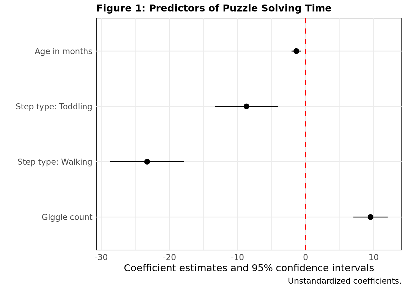
6 Figure 1. Coefficient plot

Using the mixed-effects model 2 (without interaction), we generate a coefficient plot that shows point estimates and confidence intervals. Modelplot function accepts same kinds of objects and arguments as the modelsummary function, and we can also customize the plot like any other ggplot object.

# List coefficients for the figure (rename + reorder) 
# here we plot only main effects for simplicity
coef_map <- c(
  "agemonths" = "Age in months",
  "steptypeToddling" = "Step type: Toddling",
  "steptypeWalking" = "Step type: Walking",
  "gigglecount" = "Giggle count"
)

# Create a coefficient plot
fig1 <- modelplot(
  model2,
  coef_map = rev(coef_map), # rev() reverses list order
  coef_omit = "Intercept", # omit Intercept
  color = "black"
) +
  geom_vline(
    xintercept = 0,
    color = "red",
    linetype = "dashed",
    linewidth = .75 ) + # red 0 line
  theme(
    panel.background = element_rect(fill = "white"), # Ensure background is white
    plot.background = element_rect(fill = "white", color = NA), # No border
    text = element_text(family = "sans-serif", color = "black"), # sans-serif fonts like Arial
    plot.title = element_text(size = 12, face = "bold"), # Title in bold
    plot.caption = element_text(size = 10), # Smaller text for caption
    axis.title = element_text(size = 12), # Axis titles
    axis.text = element_text(size = 10), # Axis text
    legend.title = element_text(size = 12), # Legend title
    legend.text = element_text(size = 10) # Legend text
  ) +
  labs(title = "Figure 1: Predictors of Puzzle Solving Time",
       caption = "Unstandardized coefficients.")

# Export fig1 to a PNG file
ggsave(
  here("05-outputs/figures/fig1-coefs.png"),
  fig1,
  width = 8,
  height = 6,
  dpi = 300
)

Preview the coefficient plot

7 The report package for automatic reports

The report package produces automatic reports of models and tests, following best practices guidelines (APA). The report() function creates a textual narrative of the results and report_table creates - a results table. A short tutorial video

For the demo, we will use the linear model and the full mixed model we created earlier.

# Generate narrative report from the linear model
report(model_lm)

We fitted a linear model (estimated using OLS) to predict puzzletime with
agemonths, sleephours and steptype (formula: puzzletime ~ agemonths +
sleephours + steptype). The model explains a statistically significant and
substantial proportion of variance (R2 = 0.91, F(4, 295) = 706.44, p < .001,
adj. R2 = 0.90). The model's intercept, corresponding to agemonths = 0,
sleephours = 0 and steptype = Crawling, is at 75.32 (95% CI [71.27, 79.38],
t(295) = 36.55, p < .001). Within this model:

  - The effect of agemonths is statistically significant and negative (beta =
-3.14, 95% CI [-3.32, -2.96], t(295) = -34.54, p < .001; Std. beta = -0.63, 95%
CI [-0.67, -0.60])
  - The effect of sleephours is statistically significant and positive (beta =
4.09, 95% CI [3.89, 4.29], t(295) = 40.41, p < .001; Std. beta = 0.73, 95% CI
[0.69, 0.76])
  - The effect of steptype [Toddling] is statistically significant and negative
(beta = -5.12, 95% CI [-6.47, -3.76], t(295) = -7.42, p < .001; Std. beta =
-0.33, 95% CI [-0.42, -0.24])
  - The effect of steptype [Walking] is statistically significant and negative
(beta = -10.52, 95% CI [-11.84, -9.20], t(295) = -15.73, p < .001; Std. beta =
-0.68, 95% CI [-0.77, -0.60])

Standardized parameters were obtained by fitting the model on a standardized
version of the dataset. 95% Confidence Intervals (CIs) and p-values were
computed using a Wald t-distribution approximation.

# Generate results table as a flextable
set_flextable_defaults(na_str = "") # Remove NA strings
report_table(model_lm) %>% as.data.frame() %>% as_flextable()

Parameter	Coefficient	CI	CI_low	CI_high	t	df_error	p	Std_Coefficient	Std_Coefficient_CI_low	Std_Coefficient_CI_high	Fit
character	numeric	numeric	numeric	numeric	numeric	integer	numeric	numeric	numeric	numeric	numeric
(Intercept)	75.32	0.95	71.27	79.38	36.55	295	0	0.35	0.28	0.41
agemonths	-3.14	0.95	-3.32	-2.96	-34.54	295	0	-0.63	-0.67	-0.60
sleephours	4.09	0.95	3.89	4.29	40.41	295	0	0.73	0.69	0.76
steptype [Toddling]	-5.12	0.95	-6.47	-3.76	-7.42	295	0	-0.33	-0.42	-0.24
steptype [Walking]	-10.52	0.95	-11.84	-9.20	-15.73	295	0	-0.68	-0.77	-0.60
AIC											1,795.01
AICc											1,795.30
BIC											1,817.23
R2											0.91
n: 12

# You may add further steps to customize the table...

# Generate narrative report from mixed-effects model, shorten with summary() 
report(model3) %>% summary()

We fitted a linear mixed model to predict puzzletime with agemonths, steptype
and gigglecount. The model included babyid as random effect. The model's total
explanatory power is substantial (conditional R2 = 0.86) and the part related
to the fixed effects alone (marginal R2) is of 0.54. The model's intercept is
at 63.77 (95% CI [37.42, 90.12]). Within this model:

  - The effect of agemonths is statistically significant and negative (beta =
-1.35, 95% CI [-2.07, -0.64], t(291) = -3.72, p < .001, Std. beta = -0.27)
  - The effect of steptype [Toddling] is statistically non-significant and
negative (beta = -1.75, 95% CI [-28.13, 24.62], t(291) = -0.13, p = 0.896, Std.
beta = -0.58)
  - The effect of steptype [Walking] is statistically significant and negative
(beta = -28.82, 95% CI [-54.54, -3.11], t(291) = -2.21, p = 0.028, Std. beta =
-1.55)
  - The effect of gigglecount is statistically significant and positive (beta =
9.18, 95% CI [2.07, 16.28], t(291) = 2.54, p = 0.012, Std. beta = 0.56)
  - The effect of steptype [Toddling] × gigglecount is statistically
non-significant and negative (beta = -1.93, 95% CI [-10.08, 6.22], t(291) =
-0.47, p = 0.642, Std. beta = -0.12)
  - The effect of steptype [Walking] × gigglecount is statistically
non-significant and positive (beta = 1.36, 95% CI [-6.31, 9.02], t(291) = 0.35,
p = 0.727, Std. beta = 0.08)

# Generate results table as a flextable 
report_table(model3) %>% as.data.frame() %>% as_flextable()  

Parameter	Coefficient	CI	CI_low	CI_high	t	df_error	p	Effects	Group	Std_Coefficient	Std_Coefficient_CI_low	Std_Coefficient_CI_high	Fit
character	numeric	numeric	numeric	numeric	numeric	integer	numeric	character	character	numeric	numeric	numeric	numeric
(Intercept)	63.77	0.95	37.42	90.12	4.76	291	0.00	fixed		0.69	0.34	1.05
agemonths	-1.35	0.95	-2.07	-0.64	-3.72	291	0.00	fixed		-0.27	-0.42	-0.13
steptype [Toddling]	-1.75	0.95	-28.13	24.62	-0.13	291	0.90	fixed		-0.58	-0.99	-0.16
steptype [Walking]	-28.82	0.95	-54.54	-3.11	-2.21	291	0.03	fixed		-1.55	-1.98	-1.11
gigglecount	9.18	0.95	2.07	16.28	2.54	291	0.01	fixed		0.56	0.13	1.00
steptype [Toddling] × gigglecount	-1.93	0.95	-10.08	6.22	-0.47	291	0.64	fixed		-0.12	-0.62	0.38
steptype [Walking] × gigglecount	1.36	0.95	-6.31	9.02	0.35	291	0.73	fixed		0.08	-0.39	0.55
	5.68	0.95						random	Residual
	8.39	0.95						random	babyid
n: 16

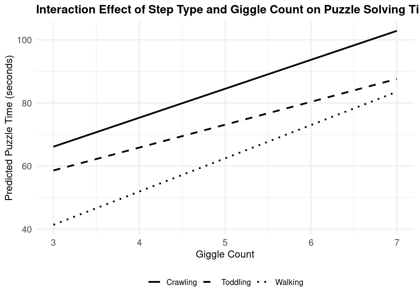
8 Figure 2. Interaction plot

Finally, we generate a interaction plot based on the mixed-effects model 3. We use the predict() function to generate predicted values for the interaction between age and step type. We then use ggplot to create the plot.

# Prepare data for prediction, focusing on steptype and gigglecount interaction
predict_data_interaction <- expand.grid(
  agemonths = mean(babysteps$agemonths),  # Use mean age to isolate the interaction effect
  steptype = unique(babysteps$steptype),
  gigglecount = seq(min(babysteps$gigglecount), max(babysteps$gigglecount), length.out = 100),
  babyid = unique(babysteps$babyid)[1]
)

# Predict puzzletime using model3 for the interaction between steptype and gigglecount
predict_data_interaction$puzzletime_pred <- predict(model3, newdata = predict_data_interaction, re.form = NA) 

# Adjusting the plot for black and white APA style
interaction_plot <- ggplot(predict_data_interaction, aes(x = gigglecount, y = puzzletime_pred, group = steptype)) +
  geom_line(aes(linetype = steptype), linewidth = 1) +  
  theme_minimal(base_size = 12) + 
  theme(
    legend.title = element_blank(),  
    legend.position = "bottom",  
    plot.title = element_text(face = "bold", size = 14),  
    axis.title = element_text(size = 12),  
    axis.text = element_text(size = 11) 
  ) +
  labs(
    title = "Interaction Effect of Step Type and Giggle Count on Puzzle Solving Time",
    x = "Giggle Count",
    y = "Predicted Puzzle Time (seconds)"
  ) +
  scale_linetype_manual(values = c("solid", "dashed", "dotted"))

# Export the interaction_plot to a PNG file
ggsave(
  filename = here("05-outputs/figures/fig2-interaction.png"),
  plot = interaction_plot,  
  width = 8,
  height = 6,
  dpi = 300,
  bg = "white"  # Ensure a white background 
)

message("Outputs saved in your output -folder") 

Outputs saved in your output -folder

# Preview the interaction plot
interaction_plot

9 Beyond the examples

There are plenty of ways to make tables beyond Modelsummary and Flextable, and many ways to refine the outputs. Check out Resources page for more alternatives of adjust the examples to your own style. Note that the examples shown are just starting points. This was not a tutorial for statistical analyses, as the focus was on creating reproducible tables and figures.

To follow the full tutorial, next step is Preparing code and data for sharing